

[물리학특수연구]ARPES data noise reduction based on autoencoder
오토인코더 기반의 ARPES 데이터 노이즈 감소
목차
- 들어가며
- ARPES data 이해하기
- EDA & 전처리
- Training
- 포스터
- 참고
1. 들어가며
물리학특수연구를 진행합니다. (23.05 ~ 23.06.)
연구 목표 : ARPES 데이터를 활용하여 280K 온도에서 수집한 ARPES 데이터와 학습 데이터셋의 무작위 생성을 활용하여 과적합을 방지하면서 신경망을 효과적으로 학습시켜 고체의 특성을 이해하는 데 기여한다.
2. ARPES data 이해하기
ARPES는 광전효과를 기반으로 합니다.
광전효과
광전효과 : 금속 등의 물질이 한계 진동수(문턱 진동수)보다 큰 진동수를 가진 (따라서 높은 에너지를 가진) 전자기파를 흡수했을 때 전자를 내보내는 현상이다. 이 때 방출되는 전자를 **광전자**라 하는데, 보통 전자와 성질이 다르지는 않지만 빛에 의해 방출되는 전자이기 때문에 붙여진 이름이다.

[이미지 출처: https://ko.wikipedia.org/wiki/광전효과]
ARPES
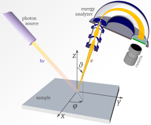
ARPES : 물질의 밴드구조를 직접적으로 관측하는 장비 (angle resolved photoemission spectroscopy - 각도 분해 광전자 분광법)
[이미지 출처:https://fr.wikipedia.org/wiki/Spectroscopie_photo%C3%A9lectronique_r%C3%A9solue_en_angle]
-간단설명-
1) ARPES를 사용하여 감지된 각 전자의 운동 에너지 $E_k$과 방출 각도 $(θ, φ)$를 기록합니다.
2) $E_k$와 $(θ, φ)$를 가지고 운동학적 특성을 이용하여 전자가 물질로부터 방출되기 전에 가지고 있던 결합 에너지 $E_B$와 결정운동량 $ħk$를 추정할 수 있습니다.
3) 바로 $E_B$와 $ħk$를 가지고 조합하여 만든 밴드 구조를 통해 고체의 성질(정보)을 알 수 있습니다.
3. EDA & 전처리
다음은 ARPES 실험 데이터를 가져와 분석하는 코드입니다.
모듈 가져오기
import matplotlib.pyplot as plt
import numpy as np
import pandas as pd
from scipy.interpolate import interp2d
CSV 파일 읽고 전치
data = np.genfromtxt('Cut280K_rNx.csv', delimiter=',')
matrix = np.transpose(data)
로우데이터 시각화
plt.imshow(matrix,origin='lower')
plt.xlabel('theta (cell)')
plt.ylabel('Kinetic Energy (cell)')
plt.colorbar() #옆에 컬러바
상수 정의
h = 6.626e-34 # Planck constant (m^2 kg/s)
hbar = h/(2*(np.pi)) # Dirac's constant
m = 9.109e-31 # electron mass (kg)
hv = 29 # 빛의 에너지  (eV)
wf = 4.43 # 일함수 (eV)
matrix 행(x축), 열(y축) 정보
delta_ke = 0.001 # kinetic Energy(eV)의 delta값
start_ke = 23.885 #kinetic Energy(eV)의 시작값
ke_unit = 'eV'
kinetic_energy = np.linspace(start_ke, start_ke + delta_ke * matrix.shape[0], matrix.shape[0])

delta_theta = 0.041096 # 각도(Θ)의 delta값
start_theta = -16.3795 # 각도(Θ)의 시작값
theta_unit = 'slit deg'
theta = np.linspace(start_theta, start_theta + delta_theta * matrix.shape[1], matrix.shape[1])
kinetic_energy와 theta 그래프 그리기
fig, ax = plt.subplots()
im = ax.imshow(matrix, extent=[theta.min(), theta.max(), kinetic_energy.min(), kinetic_energy.max()], aspect='auto', cmap='jet',origin='lower',interpolation='nearest')
ax.set_xlabel('theta ({0})'.format(theta_unit))
ax.set_ylabel('kinetic Energy ({0})'.format(ke_unit))
cbar = fig.colorbar(im)
cbar.set_label('intensity')
Binding Energy(eV) 계산
$$E_k = hν − φ − E_B 이므로$$ $$E_k − hν − φ = − E_B $$
- $hν$ : 빛 에너지
- $φ$ : 샘플 표면 작용함수(surface work function) 즉, 일함수
- $E_k$ : 광전자 운동 에너지
- $E_B$ : 전자가 방출되기 전에 가지고 있던 결합 에너지
- +) $E_k − hν − φ$ 를 $E − E_F$ 로 표현하기도 한다.
binding_energy = hv - wf - kinetic_energy
binding_energy = (-1)*binding_energy
# − E_B 즉, E − E_F를 축으로 사용한다.
K 계산
$$ħk_{||} = \sqrt {2mE_k}sin{θ} 이므로$$ $$k_{||} = \frac{\sqrt {2mE_k}}{ħ}sin{θ}$$
-
$ħK_{||}$ : 표면 평면에 대한 운동량
-
$ħ$ : Dirac's constant
-
$K_{||}$ : 파동수 m^{-1}
-
$m$ : 전자 질량 (kg)
-
$E_k (J) = $E_k (eV)$ * 1.602176634e-19 : 광전자 운동 에너지 (J)
#단위 변환 (eV -> J)
kinetic_energy_J = kinetic_energy * 1.602176634e-19
다만 K가 kinetic_energy와 theta 두 변수에 영향을 받기 때문에 2차원 배열입니다.
최종적으로 학습시킬 데이터는 binding_energy,K에 대한 intensity를 나타낸 2차원 데이터이기 때문에 2차원인 K를 그래프의 축으로 할 수가 없습니다. 즉, 1차원의 K를 새롭게 만들어야 합니다.

이때 K와 theta는 동일하게 대응하면 안됩니다.
만약 theta를 기준으로 하나의 theta에 대응하는 K와 각 kinetic_energy에 해당하는 intesnsity를 구하는 식으로 그래프를 만들면 theta가 sin함수 안에 있기 때문에 K의 간격이 점점 좁아져 0°에서 멀어질수록 그래프는 찌그러지기 될것입니다.
그렇기 때문에
- 양쪽을 kinetic_energy의 최댓값과 theta 양끝값을 대입해 구하고 그 사이를 균등한 간격으로 linspace합니다.
- 새롭게 만든 각 K의 해당하는 kinetic_energy와 theta는 기존 데이터에 없기 때문에 주변값들을 활용하여 보간해야합니다.
theta = np.linspace(start_theta, start_theta + delta_theta * matrix.shape[1], matrix.shape[1])
K_first = np.sqrt(2*m*max(kinetic_energy_J)) * np.sin(np.deg2rad(start_theta)) / hbar
K_last = np.sqrt(2*m*max(kinetic_energy_J)) * np.sin(np.deg2rad(max(theta))) / hbar
K = np.linspace(K_first, K_last, theta.size)
K=K*(10**(-10)) # 단위 m -> Å

# 2차원 보간 함수 생성
interp_func = interp2d(K, binding_energy, matrix, kind='linear') # kind = 'linear': 선형 보간, 'cubic': 3차 스플라인 보간, 'quintic': 5차 스플라인 보간

# 2차원 보간 함수를 이용하여 보간된 새로운 행렬 생성
interp_EB_K_matrix = interp_func(K, binding_energy)
코드를 보면 k 양쪽끝을 구하고 theta개수만큼 linspace하는데 theta개수만큼 만드는 이유는
- 개수를 늘리면 보간해야하는 데이터가 많아져 동시에 정확하지 않은 데이터가 많아질 확률이 올라가고,
- 개수를 줄이면 결국 가로축의 개수가 적어진다는 의미이므로 해상도가 낮아지기 때문입니다.
binding_energy와 K 그래프 그리기
fig, ax = plt.subplots()
im = ax.imshow(interp_EB_K_matrix , aspect='auto',cmap='jet',origin='lower',extent=[K[0],K[-1] , binding_energy[0], binding_energy[-1]])
ax.set_xlabel('K (Å$^{-1}$)')
ax.set_ylabel(' $E-E_F$ ({0})'.format(ke_unit))
cbar =fig.colorbar(im)
cbar.set_label('intensity')
CSV 파일로 저장
# kinetic_energy와 theta 그래프 CSV 파일로 저장
df = pd.DataFrame(matrix, columns=theta, index=kinetic_energy)
df.columns.name = 'theta ({0})'
df.index.name = 'Kinetic Energy ({0})'.format(ke_unit)
df.to_csv('Ek_theta_matrix.csv')

# binding_energy와 K 그래프 CSV 파일로 저장
df = pd.DataFrame(interp_EB_K_matrix , columns=K, index=binding_energy)
df.columns.name = 'K (Å$^{-1}$)'
df.index.name = '$E-E_F$ ({0})'.format(ke_unit)
df.to_csv('interp_Eb_K_matrix.csv')
데이터셋 구성
Data Augmentation 위와 같은 방식으로 처리된 TaSe2_GK, Cut280K_rNx, WSe2를 노이즈 입혀 각 4개씩만 plot해보았습니다.
import matplotlib.pyplot as plt
import numpy as np
from scipy.interpolate import interp2d
import torch
import torch.nn as nn
import torch.optim as optim
from torch.utils.data import DataLoader, Dataset

import matplotlib.pyplot as plt
import numpy as np
from scipy.interpolate import interp2d
import torch
import torch.nn as nn
import torch.optim as optim
from torch.utils.data import DataLoader, Dataset

class ARPESPlotter:
    def __init__(self, csv_file, start_be, delta_be, start_K, delta_K):
        self.csv_file = csv_file
        self.start_be = start_be
        self.delta_be = delta_be
        self.start_K = start_K
        self.delta_K = delta_K
        self.matrix = None
        self.new_matrix = None
        self.new_K = None
        self.new_binding_energy = None
        self.original_image = None
        self.normalized_matrix = None
        self.augmented_noisy_images = []

    def read_csv_file(self):
        # CSV 파일 읽기
        data = np.genfromtxt(self.csv_file, delimiter=',')
        self.matrix = np.transpose(data)

    def make_new_matrix(self):
        # 데이터 변경 (시작값과 간격값 적용)
        binding_energy = np.linspace(
            self.start_be,
            self.start_be + self.delta_be * self.matrix.shape[0],
            self.matrix.shape[0]
        )
        K_unit = '(Å$^{-1}$)'
        K = np.linspace(
            self.start_K,
            self.start_K + self.delta_K * self.matrix.shape[1],
            self.matrix.shape[1]
        )
        # 2차원 보간 함수 생성
        interp_func = interp2d(K, binding_energy, self.matrix, kind='linear')
        # 새로운 K, binding_energy 생성
        self.new_K = np.linspace(K.min(), K.max(), 600)
        self.new_binding_energy = np.linspace(binding_energy.min(), binding_energy.max(), 600)
        # 새로운 K와 binding_energy에 따른 matrix 생성
        self.new_matrix = interp_func(self.new_K, self.new_binding_energy)
        nan_mask = np.isnan(self.new_matrix)
        self.new_matrix = np.nan_to_num(self.new_matrix, copy=False)

    def normalize_matrix(self):
        # 행렬을 0~1 범위로 정규화
        self.normalized_matrix = (self.new_matrix - np.min(self.new_matrix)) / (np.max(self.new_matrix) - np.min(self.new_matrix))

    def augment_noisy_images(self, mean, stddev, num_aug):
        # 가우시안 노이즈를 사용한 데이터 증강
        num_augmented_images = num_aug
        for i in range(num_augmented_images):
            np.random.seed(i)  # 시드 값을 반복문 변수 i로 설정
            augmented_noisy_image = self.normalized_matrix + np.random.normal(mean, stddev, self.normalized_matrix.shape)
            self.augmented_noisy_images.append(augmented_noisy_image)

    def plot_augmented_noisy_image(self):
        num_plots = len(self.augmented_noisy_images)
        fig, axes = plt.subplots(nrows=1, ncols=num_plots, figsize=(30, 5))

        for i in range(num_plots):
            im = axes[i].imshow(
                self.augmented_noisy_images[i],
                extent=[self.new_K[0], self.new_K[-1], self.new_binding_energy[0], self.new_binding_energy[-1]],
                aspect='auto',
                cmap='jet',
                origin='lower'
            )
            axes[i].set_xlabel('K (Å$^{-1}$)')
            axes[i].set_ylabel('$E-E_F $ (eV)')
            cbar = fig.colorbar(im, ax=axes[i])
            cbar.set_label('Intensity')

        plt.tight_layout()
        plt.show()
# CSV 파일 경로 및 파일명 리스트
csv_files = ['/content/drive/MyDrive/ARPES/TaSe2_GK.csv', '/content/drive/MyDrive/ARPES/TaSe2_MK.csv', '/content/drive/MyDrive/ARPES/WSe2.csv']

# 시작값과 간격값 설정
start_be = [-0.28271, -0.316606, -2.09679]  # 파일별 시작값
delta_be = [0.0005, 0.0005, 0.00159001]  # 파일별 간격값
start_K = [-0.755169, -0.449906, -0.578732]  # 파일별 시작값
delta_K = [0.00138108, 0.00140804, 0.00166317]  # 파일별 간격값
gathering_images = []  # Initialize the list to gather augmented images

for m in range(len(csv_files)):
    arpes = ARPES(csv_files[m], start_be[m], delta_be[m], start_K[m], delta_K[m])
    arpes.read_csv_file()
    arpes.make_new_matrix()
    arpes.normalize_matrix()
    arpes.augment_noisy_images(mean=0, stddev=0.01, num_aug=3)
    gathering_images.append(arpes.augmented_noisy_images)  # Append the augmented images
num_plots = sum(len(images) for images in gathering_images)


num_rows = 3
num_cols = 3


fig, axes = plt.subplots(nrows=num_rows, ncols=num_cols, figsize=(15, 10))


axes = axes.flatten()


for idx, images in enumerate(gathering_images):
    for i, image in enumerate(images):

        subplot_idx = idx * num_cols + i


        im = axes[subplot_idx].imshow(
            image,
            extent=[arpes.new_K[0], arpes.new_K[-1], arpes.new_binding_energy[0], arpes.new_binding_energy[-1]],
            aspect='auto',
            cmap='jet',
            origin='lower'
        )
        axes[subplot_idx].set_xlabel('K (Å$^{-1}$)')
        axes[subplot_idx].set_ylabel('$E-E_F$ (eV)')
        cbar = fig.colorbar(im, ax=axes[subplot_idx])
        cbar.set_label('Intensity')


for i in range(len(gathering_images), num_rows * num_cols):
    axes[i].axis('off')


plt.tight_layout()
plt.show()
변경사항 수정 예정
4. training
import torch
import torch.nn as nn
import torch.optim as optim

# 오토인코더 모델 정의
class Autoencoder(nn.Module):
    def __init__(self):
        super(Autoencoder, self).__init__()

        # 인코더 정의
        self.encoder = nn.Sequential(
            nn.Conv2d(1, 16, kernel_size=3, stride=1, padding=1),
            nn.ReLU(),
            nn.MaxPool2d(kernel_size=2, stride=2)
        )

        # 디코더 정의
        self.decoder = nn.Sequential(
            nn.ConvTranspose2d(16, 1, kernel_size=2, stride=2),
            nn.Sigmoid()
        )

    def forward(self, x):
        encoded = self.encoder(x)
        decoded = self.decoder(encoded)
        return decoded

# 오토인코더 모델 인스턴스 생성
autoencoder = Autoencoder()

# 옵티마이저와 손실 함수 정의
criterion = nn.MSELoss()
optimizer = optim.Adam(autoencoder.parameters(), lr=0.001)

# 학습 설정
num_epochs = 100

# 저장할 체크포인트 파일 경로
checkpoint_path = "autoencoder_checkpoint.pth"

# 이전에 저장된 체크포인트가 있으면 로드
try:
    checkpoint = torch.load(checkpoint_path)
    autoencoder.load_state_dict(checkpoint['model_state_dict'])
    optimizer.load_state_dict(checkpoint['optimizer_state_dict'])
    start_epoch = checkpoint['epoch']
    print(f"Loaded checkpoint from epoch {start_epoch}")
except FileNotFoundError:
    start_epoch = 0

# 훈련 루프
for epoch in range(start_epoch, num_epochs):
    running_loss = 0.0

    # 훈련 데이터셋에 대해 루프 실행
    for clean_images, noisy_images in data_loader:
        # 입력 데이터 정의
        inputs = noisy_images

        # 입력 데이터에 대한 출력 계산
        outputs = autoencoder(inputs)

        # 손실 계산
        loss = criterion(outputs, clean_images)

        # 역전파 및 가중치 업데이트
        optimizer.zero_grad()
        loss.backward()
        optimizer.step()

        # 손실 누적
        running_loss += loss.item()

    # 에포크마다 손실 출력
    epoch_loss = running_loss / len(data_loader)
    print(f"Epoch {epoch+1}/{num_epochs}, Loss: {epoch_loss:.4f}")

    # 중간 체크포인트 저장
    checkpoint = {
        'epoch': epoch + 1,
        'model_state_dict': autoencoder.state_dict(),
        'optimizer_state_dict': optimizer.state_dict()
    }
    torch.save(checkpoint, checkpoint_path)


# 학습된 오토인코더 모델을 사용하여 테스트 데이터셋의 노이즈 제거
clean_images = []
for noisy_image in test_noisy_images:
    # 텐서로 변환
    noisy_image = torch.FloatTensor(noisy_image[np.newaxis, np.newaxis, :, :])

    # 노이즈 제거
    clean_image = autoencoder(noisy_image)

    # 텐서를 넘파이 배열로 변환
    clean_image = clean_image.detach().numpy()[0, 0, :, :]

    # 정규화 역변환
    #clean_image = (clean_image * (np.max(test_dataset.new_matrix) - np.min(test_dataset.new_matrix))) + np.min(test_dataset.new_matrix)

    # 결과 저장
    clean_images.append(clean_image)

# 테스트 데이터셋의 노이즈 제거 결과 확인
for clean_image in clean_images:
    plt.imshow(
        clean_image,
        #extent=[test_dataset.new_K[0], test_dataset.new_K[-1], test_dataset.new_binding_energy[0], test_dataset.new_binding_energy[-1]],
        aspect='auto',
        cmap='jet',
        origin='lower'
    )
    #plt.xlabel('K (Å$^{-1}$)')
    #plt.ylabel('$E-E_F $ (eV)')
    #plt.colorbar(label='Intensity')
    plt.show()
변경 사항 수정 예정 TaSe2_MK
5. 정량적 평가 지표
import cv2
import numpy as np
from skimage.metrics import structural_similarity as ssim

def calculate_metrics(original_img, noisy_img, denoised_img):
    # Calculate SSIM
    ssim_score_noisy = ssim(original_img, noisy_img, multichannel=True)
    ssim_score_denoised = ssim(original_img, denoised_img, multichannel=True)

    # Calculate PSNR
    mse_noisy = np.mean((original_img - noisy_img) ** 2)
    mse_denoised = np.mean((original_img - denoised_img) ** 2)
    psnr_noisy = 10 * np.log10(255**2 / mse_noisy)
    psnr_denoised = 10 * np.log10(255**2 / mse_denoised)

    # Calculate MSE
    mse_noisy = np.mean((original_img - noisy_img) ** 2)
    mse_denoised = np.mean((original_img - denoised_img) ** 2)

    return ssim_score_noisy, ssim_score_denoised, psnr_noisy, psnr_denoised, mse_noisy, mse_denoised

# Read the original, noisy, and denoised images
original_img = cv2.imread("/content/drive/MyDrive/ARPES/clean_3.png")
noisy_img = cv2.imread("/content/drive/MyDrive/ARPES/노이즈_3.png")
denoised_img = cv2.imread("/content/drive/MyDrive/ARPES/노이즈제거_3.png")

# Convert images to RGB format
original_img = cv2.cvtColor(original_img, cv2.COLOR_BGR2RGB)
noisy_img = cv2.cvtColor(noisy_img, cv2.COLOR_BGR2RGB)
denoised_img = cv2.cvtColor(denoised_img, cv2.COLOR_BGR2RGB)

# Calculate metrics
ssim_noisy, ssim_denoised, psnr_noisy, psnr_denoised, mse_noisy, mse_denoised = calculate_metrics(original_img, noisy_img, denoised_img)

# Print the results
print("SSIM - Noisy Image:", ssim_noisy)
print("SSIM - Denoised Image:", ssim_denoised)
print("PSNR - Noisy Image:", psnr_noisy)
print("PSNR - Denoised Image:", psnr_denoised)
print("MSE - Noisy Image:", mse_noisy)
print("MSE - Denoised Image:", mse_denoised)
전체 코드는 정리후 ipnby파일로 업로드 하겠습니다.
6. 포스터
7. 참고
-
- Angle-resolved photoemission studies of quantum materials
https://ui.adsabs.harvard.edu/abs/2021RvMP...93b5006S/abstract
-
- Deep learning-based statistical noise reduction for multidimensional spectral data
https://ui.adsabs.harvard.edu/abs/2021RScI...92g3901K/abstract
Leave a comment